These are a re-visitation of the kind of problems done in CE 561. Hopefully your newly increased proficiency in Matlab and Maple will make them easier this time.
(1) Laboratory Problem
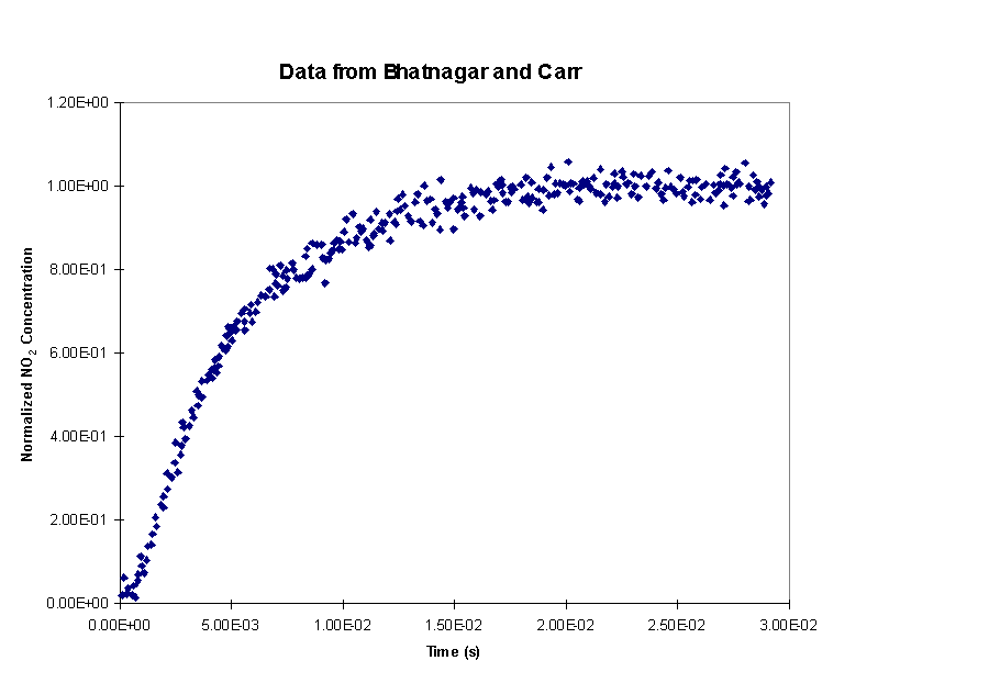
Bhatnagar and Carr (Chem. Phys. Lett., 238, 1995) studied the reaction of CF3CFHO2 with NO. The peroxy radical, CF3CFHO2, is formed in the troposphere by reaction of HFC-134a (CF3CFH2) with OH and O2. HFC-134a is the freon replacement that is currently used in automobile air conditioners. The reaction of CF3CFHO2 with NO is an important step in the degradation of HFC-134a in the troposphere. It is important that this compound is degraded in the troposphere so that it does not reach the stratosphere where it could release fluorine atoms that would contribute to ozone destruction. The rate parameters for the reaction studied in this work are needed for atmospheric models that include HFC-134a. Policy decisions about the use of different freon replacements are based (at least partially) on the predictions of these atmospheric models.
In their experiments, Bhatnagar and Carr initiated the reaction by photolyzing Cl2 to produce Cl atoms that reacted with the HFC-134a to rapidly produce the peroxy radical (CF3CFHO2). The reaction under study
CF3CFHO2 + NO ® CF3CFHO + NO2
then occurred, followed by subsequent reactions
of the oxy radical, CF3CFHO. They followed the progress of the
above reaction by measuring the concentration of NO2 using time
resolved mass spectrometry. The proposed reaction mechanism and rate coefficients
at experimental conditions (for all reactions except the one under study)
are
| Reaction | Rate Coefficient |
| (1) Cl + CF3CFH2® CF3CFH + HCl | 2.7´ 10-15 cm3 molecule-1 s-1 |
| (2) CF3CFH + O2 ® CF3CFHO2 | 2.1´ 10-12 cm3 molecule-1 s-1 |
| (3) 2 CF3CFHO2® 2 CF3CFHO + O2 | 5.0´ 10-12 cm3 molecule-1 s-1 |
| (4) CF3CFHO2 + NO ® CF3CFHO + NO2 | To be determined |
| (5) CF3CFHO ® CF3 + HCOF | 5.0´ 104 s-1 |
| (6) CF3 + O2® CF3O2 | 6.0´ 10-12 cm3 molecule-1 s-1 |
| (7) CF3O2 + NO ® CF3O + NO2 | 1.6´ 10-11 cm3 molecule-1 s-1 |
| (8) 2 CF3O2® 2 CF3O + O2 | 1.8´ 10-12 cm3 molecule-1 s-1 |
| (9) CF3O + NO ® CF2O + FNO | 4.7´ 10-11 cm3 molecule-1 s-1 |
| (10) CF3O2 + CF3O ® CF3OOOCF3 | 1.4´ 10-11 cm3 molecule-1 s-1 |
[Cl] = 4.32´ 1013 molecules cm-3
[CF3CFH2] = 2.67´ 1017 molecules cm-3
[NO] = 7.26´ 1013 molecules cm-3
[O2] = 2.3´ 1016 molecules cm-3
Note that an initial concentration of Cl atoms is given, since the photolysis of Cl2 produces these atoms on a time scale much shorter than that of the experiment.
Using the reaction mechanism presented above, apply a non-linear least squared analysis to obtain a value of the rate coefficient for reaction (4) (Bhatnagar and Carr got k4 = 1.3´ 10-11 cm3 molecule s-1). Plot the resulting model prediction along with the experimental data. Compute the sensitivity of the NO2 concentration profile to each of the rate constants in the mechanism. How does the sensitivity of the model results to the rate coefficient being measured compare to the sensitivity of the model results to the other rate coefficients? Comment on the effect of uncertainties in the other rate constants on the fitted value of the rate constant being measured.
(2) Test Problem
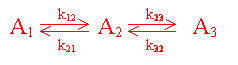
Consider the network of 1st order
reactions given by
taking place in a fixed bed reactor with significant
axial mixing. In dimensionless form, the governing equations for
this situation are given by the boundary value problem:
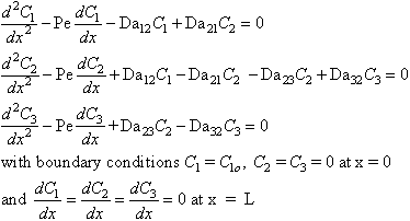
If the Peclet number is sufficiently large, then
the diffusive terms can be neglected, and the equations become the initial
value problem
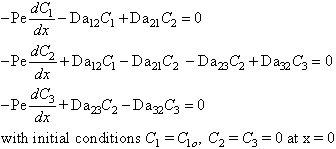
Use Maple to find an analytical solution to the
initial value problem that describes the reactor when the Peclet number
is large. Evaluate this solution for
C1o= 1, Pe = 10, Da12 =
5, Da21 = 2, Da23 = 10, Da32 = 5.
Plot the result.
Use Matlab to solve the same equations numerically, for these values of of the parameters. Confirm that you obtain the same result that you got using Maple.
Use Matlab to solve the full boundary-value-problem
(including axial dispersion) for C1o= 1, Da12 = 5,
Da21 = 2, Da23 = 10, Da32 = 5, L=1, and
values of the Peclet number ranging from Pe = 0.001 to Pe = 1000.
For Pe = 10, compare the result to the solution of the initial value problem.
Obtain this solution by discretizing the equations
using finite differences, as discussed in CE 561. The relevant lecture
notes, including an example, are given here.