Analog computing concepts are used in signal processing for many instrumentation applications and are an important aspect of continuous control system design. The strain gage conditioners you have been using this semester processing force, torque and pressure signals contain analog circuits as do the function generators. The analog to digital converters that are part of the National Instruments LabView package also use analog computing components. The derivations below are intended to describe the working principles of analog computing. Only the most basic ideas are presented.

Basic Concept

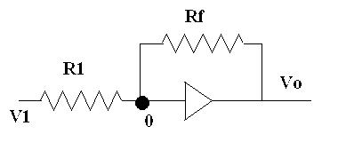
The fundamental analog computing element consists of a feedback resistor and an input resistor as shown below. The resulting simple circuit is analyzed by summing currents at the input junction point to the operational amplifier (op amp). The gain of the op amp is so high that an output voltage Vo is obtained with negligible input voltage. The input node may be considered to be at zero voltage as shown in Figure 1 below.

Figure 1
 

(1)

The summation of currents leads to the simple equation (1) for output voltage Vo in terms of the input voltage V1 and the ratio of resistances Rf/R1. Note the negative sign. All op amp circuits perform sign changes. Typically analogs are preset to have resistance ratios giving gains of 1, 0.1 or 10.

Summation

The basic anaolg circuit can be turned into a summing circuit by adding an additional input resistance as shown in Figure 2 below. Again, the summation of currents at the input junction is performed

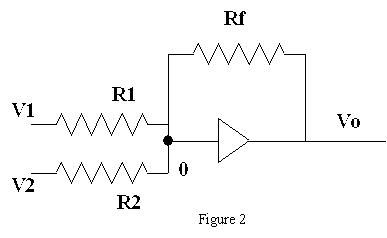
and then
 
 

and for R2 = R1,

or if Rf = R1,

Integration

An integration may be performed by inserting a capacitance element into the op amp circuit as in Figure 3 below. The integration gives the analog computer the capability to solve differential equations and simulate dynamic systems. These types of systems were once the primary way to obtain rapid dynamic solutions to differential equations modeling chemical plants, aircraft dynamics, etc. Of course, this simulation role has been very much replaced by digital computation. However, dynamic signal processing is still frequently performed in instrumentation and control loops.

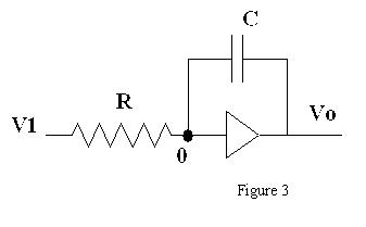
The integrator model begins with a current summation again so that

and in this way the output voltage is related to the integral of the input. The selection of R and C then defines the gain.

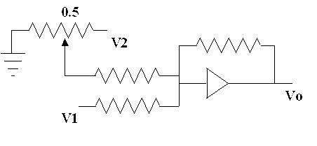
Using Potentiometers

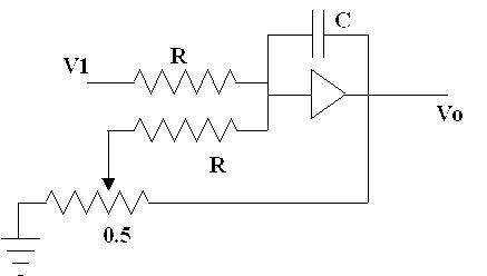
The feedback resistors and capacitors in analog computing are usually chosen to provide gains in multiples of 0.1, 1 and 10. Potentiometers are then used to make adjustments at in-between levels. For example the arrangement in Figure 4 below with all resistors equal and a pot setting of 0.5 would provide an output proportional to V1 + 0.5 V2.

Figure 4
 

Solving a Differential Equation

The circuit in Figure 5 below uses a capacitor integrator and a potentiometer to solve a differential equation. The equation (which can be derived using the current summing concept shown above) is

Of course, if RC = 1 (this is easy to arrange), the differential equation becomes

Figure 5
 

Initial Conditions

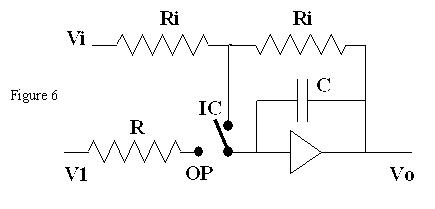
In solving differential equations, it is necessary to to be able to apply the intial conditions which define the problem?s starting point. The ability to include initial conditions is provided by "initial condition" mode and the "operate" mode of the computer. A press of a switch as shown in Figure 6 below changes between the modes. The initial condition mode sets up the differential equation?s starting conditions. The operate mode executes the solution of the equations. In the circuit below, the initial condition in the IC mode is Vo = -Vi (remember the always present sign change). If RC = 1, the operate mode then starts from the -Vi starting value and simply integrates -V1.
 

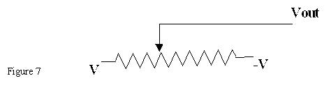
The Ungrounded Pot

On an analog computer, a potentiometer can be conveniently supplied with positive and negative voltages across the full resistance. In the case of Figure 7, the wiper arm can be set at the middle where it would provide an output of zero volts. Or, it could be moved towards either end, in one case providing a positive output voltage up to +V or in the opposite providing a negative voltage as far as -V.