The simulation of the RLC circuit transient behavior in Experiment #3 used a Matlab function for solving linear state equations. This is certainly an important capability of the Matlab package. However, Matlab contains a wide variety of numerical, analytical and plotting capabilities that continue to amaze all of us who were preparing our own computer tools before Matlab became so widely used and so powerful (this includes myself and Dr. Mook).

The example below shows a Matlab tool for solving nonlinear differential equations in state equation form. The fluid capacitance behavior apparent in Experiment #5 defines a naturally nonlinear system. The Matlab function illustrated below is "ode23". It is called by the example ".m" file TransientD.m. This file obtains a Matlab solution and also plots it alongside the experimental result. The file first reads in the Excel output file from the discharge experiment (this Excel text file must, of course, be fully trimmed of all text except for the data of interest). In this case the Excel file contains only columns representing time, flowrate and pressure and only the time and pressure information is used and plotted by Matlab.

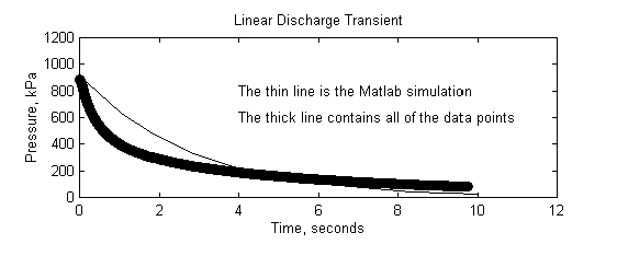
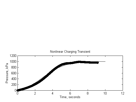
The TransientD.m file calls Matlab?s "ode23" for solving nonlinear state equations. The function ode23 is told to call "StateEqnD.m" to obtain full state equation information. This second .m file is shown on the following page as used to solve the fluid system transient with constant fluid capacitance C. The plot resulting from executing TransientD.m with StateEqnD.m as shown is included on the next page with the title "Linear Discharge Transient". To change this simulation to the nonlinear case, your equation for fluid capacitance with pressure dependence should be inserted as indicated. A response much more compatible with the experiment should then be possible. The final plot shown was obtained in a simulation of the charging transient using a nonlinear capacitor model and an appropriate value for PressApp. Notice that the simulated charge agrees very well with the experimental data.

This is the Matlab .m file "Transientd.m".

*********************************************************

load capdischtqp.txt % Loads the scaled and trimmed data file.

tdata=capdischtqp(:,1); % Defining the time data.

tdata=tdata-.25; % Response begins at 0.25 seconds.

pdata=capdischtqp(:,3); % Pressure is in the third column.

P0=[928]; % Sets the initial pressure

Tfinal=10; % Sets the integration time

[t,Pcalc]=ode23('StateEqnD',[0 Tfinal],P0); % Calls the Matlab solver

% Plotting commands

subplot(211);plot(tdata,pdata,'yo',t,Pcalc,'k')

axis([0 12 0 1200]);

title ('Linear Discharge Transient')

xlabel('Time, seconds')

ylabel('Pressure, kPa')

text(4,800,'The thin line is the Matlab simulation')

text(4,600,'The thick line contains all of the data points')

**********************************************************

This is the .m file "StateEqnD.m" for defining nonlinear state equations.

**********************************************************

function Pdot = StateEqnD(t,P)

Pdot=zeros(1,1);

R=55e06;

C=0.05e-06; %This is a constant capacitance.

%Enter your nonlinear capacitance here!

PressApp=0; % Applied pressure of zero.

Pdot(1)= ((PressApp-P(1))/R) /C; % The state equation.

***********************************************************