INTRODUCTION

This experiment continues with the study of fluid system components and considers fluid capacitance. The hydraulic capacitor studied here results from the entrapment of air in the fluid system - a typical source of capacitance in hydraulic systems. The experiment involves measuring the characteristics of the fluid capacitor and then using a mathematical representation of its capacitance to describe its behavior during a transient event. The equipment and instrumentation are essentially the same as used in Experiment 4 with the addition of the capacitor and a manually operated valve. Two basic events are to be monitored during the experiment - (1) the charge of the capacitor to a pressure approximating the supply pressure and (2) the discharge of the capacitor to the return pressure. The capacitor pressure and the capacitor flowrate are to be monitored during both of the events. The resulting data from charging the capacitor are to be used to determine the hydraulic capacitance as a function of system pressure. The transient pressure of the capacitor discharge will be modeled in Matlab and compared to the data obtained in the second part of the experiment.
 
 

EQUIPMENT SET-UP AND DATA COLLECTION

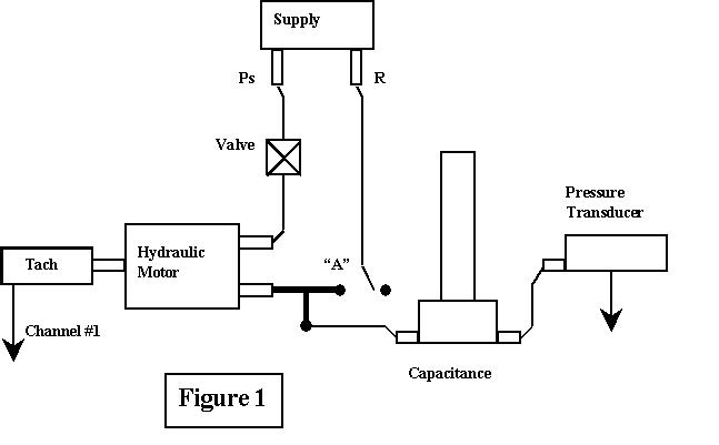
The basic laboratory apparatus is shown in Figure 1 below.
 

Pressure measurements in this experiment are made by using the differential pressure transducer in a "single-sided mode". The pressure transducer should be calibrated against the hydraulic system pressure gage at the 100 psi level (where 1 psi is 6.90 kPa). Be certain that the strain gage conditioner is zeroed and that the reference side of the pressure gage has been discharged to atmospheric pressure.

As in Experiment 4, the calibration of the tachometer/hydraulic motor arrangement for flowrate measurement depends on the displacement of the motor (0.095 cubic inches per revolution) and the tachometer gain (7 volts per 1000 rpm). Be sure that you show your calculations to determine the calibration scale factor for the pressure transducer in kPa/volt and the calibration scale factor for the flow measurement arrangement in cubic meters/sec/volt.

Charge the capacitor by setting the supply pressure of the hydraulic system to 200 psi and arranging the system as shown in Figure 1 above. The manual valve is an adjustable fluid resistance that can control the charging rate. You will need to adjust it so that the pressure increase takes place over approximately 10 seconds (to obtain a good fit on the LabView VBscope) and also so that the capacitor charges smoothly with no more than a minimal oscillation.

The actual charging process is to be performed in the arrangement of Figure 1. Begin by initially connecting the return line (at "A") to the Tee in Figure 1. Because of the high resistance of the adjustable valve, this essentially discharges the fluid capacitance and at the same time establishes a small flow through the system. Carefully (but quickly) remove the quick-disconnect return line at "A". The established flow becomes the initial charging flow of the capacitor. This flowrate increases the capacitor pressure until it approaches the supply pressure. As the capacitor pressure increases, the flowrate decreases. When the capacitor pressure becomes large enough, the hydraulic motor no longer turns and the charging flow becomes zero. You can easily discharge the capacitor pressure by reconnecting the return line at "A". You can then recharge it by disconnecting the line.

Repeat this process a few times, adjusting the valve setting (it has a numbered scale) until you have been able to capture the pressure and flow curves for a smooth charging transient over a bit less than ten seconds. Click on "single" to save it and place it in a file for Excel to be processed later.

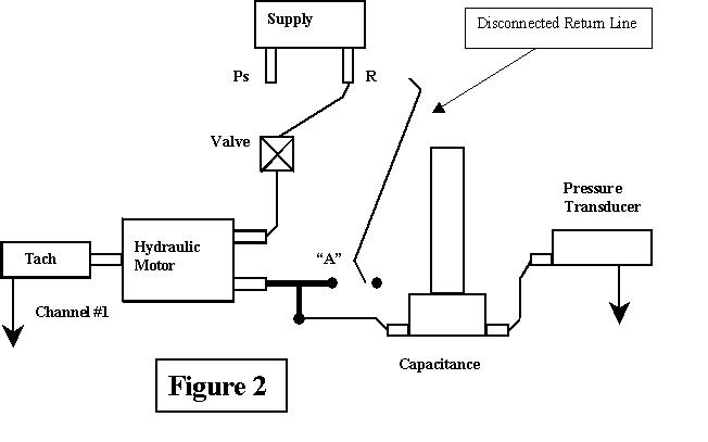
Use the arrangement of Figure 2 (next page) to obtain a discharge transient for the system. The valve setting for the charging transient should also provide a reasonable setting for the discharge transient. Note that the later portion of the capacitor discharge becomes particularly slow and may not fit completely within the ten second VBscope plot. However, you should have no difficulty capturing the most significant part of the discharge. You can repeat this charging/discharging process as necessary to obtain a nice plot but recharging the capacitor will require reconnecting your valve line to the supply pressure. It should only take a few tries to capture data for the pressure and flowrate during a discharge transient.
 

RESULTS SECTION

1. Use your charging data and calibrations to develop a properly labeled and scaled plot of the charging transient. Use Excel to plot pressure (kPa) and flowrate (cubic meters/second) vs. time. (Required plot #1.)

2. Process the charging transient data to calculate the capacitance of the fluid system based on the relation C dp/dt = q. The pressure transient can be differentiated for this calculation but this must be done carefully using (delta p / delta t) over a span of several data points. An example spreadsheet entry might take the form of (p21-p1)/(t21-t1). For entrapped air, capacitance is a function of system pressure. Obtain a properly labeled plot of your experimental capacitance C vs pressure p for your charging data. (Required plot #2.) Note that fluid capacitance may be measured in units of cubic meters per kPa.

3. At any instant, the capacitance C = V / Pabs for isothermal behavior of entrapped gas and an instantaneous gas volume V (Shearer et al., pg 188). Recall that Pabs = Pg + 101 in kPa. In terms of an initial pressure and volume, this becomes C = Pi Vi / P^2 where the pressures are again absolute, not gage. You will need to adjust your volume Vi to obtain the effective volume of air initially trapped in the system. Your calculation can be compared against your experimental results by adding a calculated curve on your C vs P plot. When you have determined a volume that gives best agreement, report the resulting volume and present your final graph of calculated and theoretical capacitance vs. pressure. (This is required plot #3.)

4. For your experimental discharge results, use Excel and your calibration data to obtain a properly labeled and scaled Excel plot of pressure and flowrate during the discharge transient. (Required plot #4.)

5. Prepare the time and pressure columns of your "discharge Excel file" so that they can be read into Matlab. Use a Matlab "ode" routine for solving the ordinary nonlinear differential equation describing the capacitor discharge processs. You can use your capacitance model with the effective volume that you determined during charging to describe the system. Also assume a linear resistance model for the valve. Compare the Matlab simulation of the discharge transient to your laboratory discharge pressure transient. Adjust the linear resistance value in your Matlab model to fit the experimental transient and show the resulting comparison of the experimental and simulated pressure transients on a Matlab plot. (Required plot #5). What is the effective linear resistance for the valve in units of kPa-seconds/cubic meter?
 
 

SPECIFIC QUESTIONS

1. The physical volume of the capacitor used in this experiment is 1 inch in diameter and 6 inches long. How does your reported volume (item #3 above) compare to this? Is this as expected? Explain.

2. It is possible to experimentally study the fluid resistance character of the adjustable valve by performing a pressure-flow test. Describe a simple experiment that would allow this to be done using the equipment that you have been working with in the lab.

3. The pressure-flow behavior of the adjustable valve may be governed by orifice flow. If this is the case, would you expect the pressure flow resistance to be linear? What would be the ideal equation defining the pressure-flow relation? Sketch the expected pressure-flow curve for orifice flow conditions.
 
 

REPORT

Individual short form reports should be submitted for this experiment (see the Web page for details). Each person must submit his/her own individual report. But you are certainly encouraged to work with your group members on the data analysis, computation, results and simulation. All of the narrative sections of the report (including theory, procedure, discussion, conclusions and written responses to questions) should be independently prepared.