INTRODUCTION
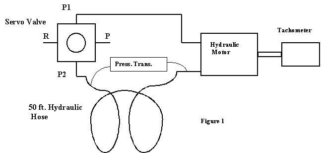
Hydraulic systems are used widely in applications where high levels of power, force or torque are required and especially if these must be delivered while supporting fast transient behavior. This experiment introduces common hydraulic system components and uses them to measure the flow resistance character of a long hydraulic hose. The basic approach begins with a signal from a function generator which activates the system. The function generator signal is amplified by a hydraulic servo amplifier which controls a two stage hydraulic servovalve. The valve movements allow the hydraulic power source to provide flow through a 50 foot long hydraulic line. The flow is instrumented by a hydraulic piston pump which is turned by the flow. A tachometer on the pump shaft allows the pump speed (and thus the flowrate) to be measured. A differential pressure transducer is connected across the long line and measures the resulting pressure drop in the line.
EQUIPMENT SET-UP AND DATA COLLECTION
The overall equipment arrangement is shown in Figure 1 below.
The servovalve connections marked P and R are connected by quick disconnect lines to the hydraulic power supply with P to the pressure side and R to the return side. The pressure transducer is a strain gage device and should be connected to the strain gage conditioner with the conditioner output displayed on channel two of the VirtualBench-Scope. The tachometer signal should be displayed on channel one. Since the gain of this tachometer is 7 volts per 1000 rpm, you should be able to connect it directly to channel one. However, if you would like to explore high flowrates and turbulent flow in the line (see question 4), the tachometer speed signal will exceed the +/- 5 volt limitation of the A/D converter and a potentiometer will be needed to reduce the signal magnitude (as was done for the motor tach in Experiment 2).
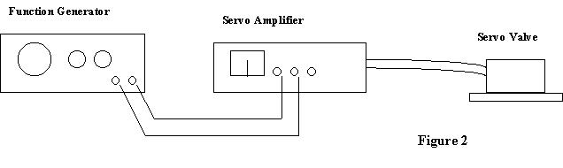
The function generator controls the servovalve through the servoamplifier as shown in Figure 2 below.
The tachometer operates as a flowrate transducer because the hydraulic pump is a positive displacement device and its volume flowrate is directly proportional to its speed. The pump displacement is provided by the manufacturer as 0.095 cubic inches per revolution. The tachometer calibration is 7 volts per 1000 rpm. Calculate the flowrate calibration scale factor in terms of cubic meters/sec/volt.
The pressure transducer should be calibrated against the pressure gage of the hydraulic supply. Connect the pressure transducer with the supply pressure applied on one side and the return connection made to the other side. Before turning on the hydraulic power unit, adjust the strain gage conditioner to balance it at zero. Turn on the hydraulic power and adjust the pressure to about 100 psi to obtain a calibration point. You may obtain additional points, also note that reversing the hydraulic connections (turning off the power first is a good idea) will give you a "negative" calibration point for the differential pressure transducer. Obtain your pressure calibration scale factor in units of KiloPascals per volt (one psi = 6.90 kPa).
With your apparatus re-assembled in the form of Figure 1, place the tach on channel one and the pressure on channel two and set the scope to free run. Set the function generator to zero amplitude with a triangular wave form and low frequency (about 0.2 Hz or less). Turn on the hydraulic power and adjust the pressure to about 200 psi. Adjust the function generator bias to close the servovalve so that there is no flow through your long hose. If the pump shows some residual slow speed - this is OK, it?s difficult to get perfect balance in hydraulic systems. But if the pump is turning considerably, ask for help in improving the balance. With the scope free running, gradually increase the triangle wave amplitude. The pressure and tach signals should increase correspondingly. When the signals are well established and the tach voltage is in the 3-4 volt range, switch your scope to the x-y plotting mode. The resulting pressure flow line defines the resistive character of the long hose and should be reasonably linear. If you see considerable hysteresis, lower the triangular wave frequency as much as practical to reduce it. Finally, capture the data by returning to time plotting and clicking on "Single". Required plot #1 is the time plot of the pressure and flowrate fluctuations, required plot #2 is the plot of pressure drop vs. flowrate. Both plot #1 and plot #2 should be completed and labeled with Excel and, of course, should be scaled into proper units of pressure and flowrate.
Place your VB-Scope in x-y plotting mode. Increase the frequency of the triangle wave and notice the plot change. At an appropriate frequency level, you should be able to see the up and down-going lines on the plot separate and take on a hysteretic appearance. When you have this clearly established, capture the data. Use Excel to scale and label the higher frequency pressure-flow plots (required plot #3 is the pressure vs. flowrate plot clearly showing hysteresis).
QUESTIONS
1. For laminar flow, plot # 2 is ideally linear. Do you have a linear plot? What effects could distort the linear character? The component equation for fluid resistance is p = Rq. Use the slope of your plot to compute the effective hose resistance in units of kPa-seconds per cubic meter.
2. From your resistance calculation above, calculate the effective viscosity of the hydraulic fluid used in the experiment. Is this a reasonable result? Considering the graph of typical hydraulic fluids shown in Figure 3, which fluid (by ISO number) matches your measured viscosity? What factors may have influenced any errors that you?ve experienced?
3. The component equation for fluid inertance is p = I dq/dt. The hysteresis form shown in your plot # 3 is largely a result of the inertance of the fluid in your long hose. Based on the inertance equation, explain the hysteresis in plot #3. Why is the hysteresis small at low frequency and why does it grow with increased frequency?
4. What do you think will happen with flowrates large enough to have turbulent flow in the hose? Would the pressure-flow plot remain essentially linear? Would it curve upward or downward with increasing flow? Reference? Explanation? Do you have any experimental result?
Figure 3