
10.1 Discussion
10.2 Loops with for and while
10.3 Tests with if Statements
10.4 Global and Local Variables Used in Functions and m-files
10.5 The Heading of a MATLAB Function
You will find that you can solve many problems in MATLAB that would require complicated FORTRAN programs with just the programs that are furnished you. Writing programs in MATLAB is quite simple for most other engineering problems. Programs are edited and stored in regular text files, but must have: .m after their names. As soon as a program is defined and saved in: the directory that MATLAB was entered from (or the user's home directory if it was activated from the Applications' menu) or the user's MATLAB directory the program can be used. Please note four important points:
1) The program is edited and saved just like any other file. This may be done in an window or any other way that is convenient for you.
2) The program must be saved in a file that has .m appended to it.
3) The program is executed in a MATLAB Command Window.
4) Only the name (without the .m suffix) is given when you want to execute the program.
One bit of advice about the programs (in MATLAB even more than in other languages): Add comments that describe what the function does and give an example of its use in another comment. This not only helps when you list the function in Unix or a text editor, it also can be a concise way to see what the function does with the help command.
You will find it most convenient to store all MATLAB programs in a single directory. If you call this directory MATLAB (and it is a subdirectory of your home directory), they will automatically be accessible to you in MATLAB no matter what directory you are in when you enter it.
MATLAB contains several flow control procedures that are similar (but not identical to) those in FORTRAN. These include FOR and WHILE (instead of DO) loops and IF statements. The form of a FOR loop is:
for k=1:n.........
(lines of program)
.........end
The lines of the program between the for and its end will be repeated n times. We can demonstrate this in a MATLAB session:

WHILE loops allow you to repeat a set of instructions until some logical condition is no longer satisfied. It's form is:
while logic.........
(lines of program)
.........end
Here is a simple example:

The usual form of an IF statement is:
if(logical).........
(lines of program)
.........end
Help applied to if shows more about the way it works:
>> help if

IF   Conditionally execute statements. The simple form is:
                IF variable, statements END
     The statements are executed if the variable has all
     non-zero elements. The variable is usually the result
     of expr rop expr where rop is ==, <, >, <=,
     >=, or ~=

     For example:

               IF I == J,
                  A(I,J) = 2;
               ELSEIF ABS(I-J) == 1,
                  A(I,J) = -1;
               ELSE
                  A(I,J) = 0;
               END
This is convenient, since it allows one to test directly to see if character strings match. Here is a simple program to make sure we understand the help description.

>> tstif2('abc','abc')
Same

>> tstif2('abc','abb')
Not the same
Unfortunately, the program can give some problems if you try to compare strings of different lengths:
>> tstif2('aaa','a')
Same

>> tstif2('abc','aa')

??? Error using ==> ==
Matrix dimensions must agree.

Error in ==> /marsh/ceng301/matlab/ceng303/tstif2.m
On line 2  ==> if a==b
To avoid this problem, you can use the function strcmp to compare character strings as in the program tstif3.

Here are the same examples shown to give problems if you simply use "==":
>> tstif3('aaa','a')
Not the same

>> tstif3('abc','aa')
Not the same
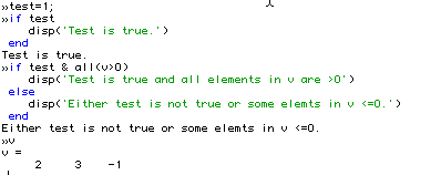
The logical test may be applied to a value that has been set in a variable or it may consist of a complex determination involving relational operations combined with logical operations. Here are examples of each:
Another set of examples begins with the program shown below. It was edited and saved as a file called root1.m with a standard editor and was then stored in my MATLAB directory so that I could always access it from any active directory. I moved it to: ~ceng301/matlab/ceng303 so others can execute the program by simply typing its name: root1. It lists as:
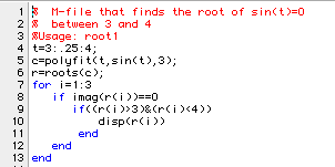
In MATLAB, I can use root1 with the following results:
>> clear
>> root1
    3.1415

>> who
Your variables are:
 c         i         r         t
The "program" is nothing more than a sequence of MATLAB instructions that you can test in a MATLAB session. The program has the advantage that you can use it over again with different data to solve similar problems. You should note that all the variables defined in the program become variables in your active workspace. This has an advantage in that they could now be used for further calculations. Its disadvantages are:
1) you can alter values of variables of the same name in your workspace,
2) you add to the number of variables and thus may make it harder to find one that you want with who.
A brief explanation of each line in the program root1is given next:
|
Line(s) |
Performs |
|
1-3 |
Comments that give the main purpose of the program and how to use it. |
|
4 |
Makes a vector called t with elements: 3 3.25 3.5 3.75 4. |
|
5 |
Finds the coefficients in a cubic that best fits sin(t) over the interval given in t . |
|
6 |
Finds the three roots of the cubic. |
|
7 |
Defines a vector with elements: 1 2 3 and starts a loop in which i takes on each of these values. |
|
8 |
Tests to see if a root is real (if not it will not be tested further). It really asks if the imaginary part of the root is 0. |
|
9 |
Tests to see if a root is in the interval (3,4). It asks if the root (known to be real) is greater than 3 and less than 4. |
|
10 |
If the root is in the interval (3,4) and is real it is listed. |
|
11 |
Marks the end of the inner test. |
|
12 |
Marks the end of the outer test. |
|
13 |
Marks the end of the for loop. |
Note that the indentation is not required, but just as in FORTRAN it helps make the program readable.
Obviously the program shown as root1 is not very useful since it is restricted to solving a single problem. We can make it much more general by changing to the format of a MATLAB function with arguments that give us the desired flexibility. Our first example of a function is shown as root2:
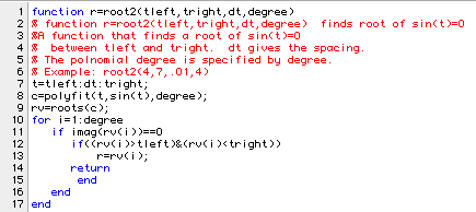
Now we can find the same answer as before by:
>> clear

>> disp(root2(3,4,.25,3))
    3.1415

>> who
Your variables are:
   degree    dt        tleft     tright
But we can also find other roots as the example in the comment suggests:
>> disp(root2(4,7,.01,4))
    6.2836
The major changes from root1 to root2 are listed below:
|
Line(s) |
Performs |
|
1 |
The heading shows that the function returns the value last put in r, and has four arguments with each argument defined. |
|
2-6 |
Comments that give the main purpose, the meanings of the arguments and an example use. |
|
7 |
Now the interval and number of points may be changed. |
|
13 |
Now the program returns the value found for the root rather than just listing it. |
We are still restricted to finding roots of a single equation: sin(t)=0. Wouldn't it be nice to be able to do this for any function? The command eval provides the means for doing exactly that as seen in the function root3 :
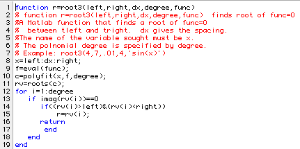
Now as we change the function specified as a character vector in the last argument of root3 we can look for the root of anything. The only changes that were required to do this were:
1) Insert line 9 to take the name we gave and assuming there is a single argument of the function, evaluate f(x) for each value of x.
2) Change line 10 to replace what was given by sin(t) with the values stored in f.
We will show it used here for our same old problem.
>> disp(root3(3,4,.25,3,'sin(x)'))
    3.1415
Note that I changed the required name of the variable sought from t to x as a transition to the usage in the secant functions: ssec1 and ssec2.
Even simple functions like root2 and root3 can have problems either in the programs or in the way they are used. A large part of using any programming language is finding out how to find errors and correct them. The next chapter will go into this in some detail.
Now let's look at the ssec1 and ssec2 functions. The first lists as:
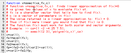
The comments explain most of what we need to understand and use it. If we execute the example lines, we see:
>> cs=[1 -2 -4.25 7.5];

>> disp(ssec1([2 3],'polyval(c,x)',cs))
    2.2105
The function has the values as seen in the next lines at the two points: 2 and 3.
>> disp(polyval(cs,[2 3]))
   -1.0000    3.7500
A linear fit of the data found would be:
>> disp(polyfit([2 3],[-1 3.75],1))
    4.7500  -10.5000
or: 4.75x-10.5
If we set this equal to 0 and solve for x we get: 2.2105 just as ssec1 found. If we try ssec1 again, but change the interval to (3, 2.2105) and then repeat as ssec2 does, we should get closer to our root.
>> disp(ssec1([3 2.2105],'polyval(c,x)',cs))
    2.3586

>> disp(ssec1([2.2105 2.3586],'polyval(c,x)',cs))
    2.5912
The process shown above is what ssec2 uses to iterate for a solution. A listing of the function is shown next:
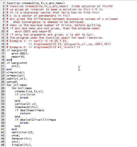

Note some of the very important features in this trial and error program. It will always terminate since it keeps track of how many times it executes ssec1. It anticipates that it may not succeed and tells the user if it does not find a root to the desired accuracy. It can accept 2, 3 or 5 arguments. If two are given, they must specify the interval to be searched and the function of x. The third argument can be a vector of constants and the last two are the allowed error and number of iterations. If the vector of constants is not given, it is set to a null vector. If the error and iteration parameters are not supplied, they are set to default values. The program was demonstrated in the examples chapter so we will not repeat that here.
10.4 Global and Local Variables Used in Functions and
m-files
In MATLAB all variables are assumed to be local in a function unless they are explicitly declared to be global in that function. If those same variables are to be used in another function, or in the command window, they must also be declared there. Thus data (unless declared global in that function) must be passed in the argument list of the function as we did with the polynomial coefficients in the functions ssec1 and ssec2. However all variables defined in the MATLAB command window are readily used in MATLAB m-files which are not functions. Here is a short m-file called tglob1 to show what happens in using such a file:

Here is a session used with tglob1:
>> a1=100.35;

>> v1=[2 5 1.2];

>> v2=[55 2 1];

>> tglob1

Here are some variables that you have defined.
a1 =
  100.3500
v1 =
    2.0000    5.0000    1.2000

Now give a vector that you have defined. v2

v2 =
    55     2     1
If we make the variables global, it has no effect on the use of them in the m-file:
>> global a1 v1 v3
Warning: Future versions of MATLAB will
require that you declare a variable to be
global before you use that variable.
Warning: Future versions of MATLAB will
require that you declare a variable to be
global before you use that
variableevising this example, first
clear the variables a1, v1, v2, and v3.
>> clear a1 v1 v2 v3
Now declare a1, v1, and v3 as global variables and re-enter the values for a1, v1, and v2.
>> global a1 v1 v3
>> a1=100.35;
>> v1=[2 5 1.2];
>> v2=[55 2 1];
Now enter the value for v3 and run tglob1.
>> v3=[4 4 4];

>> tglob1

Here are some variables that you have defined.
a1 =
  100.3500
v1 =
    2.0000    5.0000    1.2000

Now give a vector that you have defined. v3
v2 =
    4     4     4

>> v2

v2 =
     4     4     4
Note that the variable v2 has been reset as a result of this execution in the command window workspace.
In a function, the situation is quite different. The m-file tglob2 is similar to tglob1, but its heading shows that we have defined it to be a function:

We will use it in a workspace that has been cleared of all variables:
>> a1=55.5;

>> v1=[1 4 2];

>> v2=[8 3 1.1];

>> tglob2

Here are some variables that you have defined.
???  Undefined function or variable 'a1'.

Error in ==> /marsh/ceng301/matlab/ceng303/tglob2.m
On line 4  ==> a1
Obviously, the function knows nothing about the variable a1 and we can anticipate that it will not know about v1 . Making them global will allow the program to associate values with the names, but only if we globalize the variables in the command window and the function. To do this, clear the variables again, declare them as global, and re-enter their values.
>> clear a1 v1 v2
>> global a1 v1
>> a1=55.5;
>> v1=[1 4 2];
>> v2=[8 3 1.1];
Now run tglob2.
>> tglob2

Here are some variables that you have defined.
??? Undefined function or variable 'a1'.

Error in ==> /marsh/ceng301/matlab/ceng303/tglob2.m
On line 4  ==> a1
In this case, the variables were globalized in the command window, but not in the function, so the function still didn't know what a1 and v1 were. If we add a global statement in the function as well, the function will work properly.

>> tglob2a

Here are some variables that you have defined.
a1 =
   55.5000
v1 =
     1     4     2
Now give a vector that you have defined.
>> v2

v2 =
     [ ]
The whole program runs, but it does not get the values we stored for v2 when it tried to put them in. The vector v2 is still defined in the command window:
>> v2

v2 =
    8.0000    3.0000    1.1000
but the function again does not know about those values. All the function knows about are variables defined internally or globally. It does not acknowledge those set in the command window.
If we try to run tglob2 and give v3 (a new vector) as the variable to be read in, we get:
>> v3=[4 4 4];

>> tglob2a

Here are some variables that you have defined.
a1 =
   55.5000
v1 =
     1     4     2

Now give a vector that you have defined. v3
??? Undefined function or variable 'v3'.
After tglob2a prints the statement: ``Now give a vector that you have defined.'' you have to give (numeric) values for the vector elements in order to to continue:
Now give a vector that you have defined. [1 1 1]

v2 =
     1     1     1
If we make v3 global, we can get it into our function. Again, clear v3, since we already referred to it. Next, declare it as global and reassign its value. Then run tglob2a
>> clear v3
>> global v3
>> v3=[4 4 4];
>> tglob2a

Here are some variables that you have defined.
a1 =
   55.5000
v1 =
     1     4     2

Now give a vector that you have defined. v3

??? Undefined function or variable 'v3'.
Of course, that is because we also need to globalize v3 as in the function, which we will now call tglob2b.
>> tglob2b

Here are some variables that you have defined.
a1 =
   55.5000
v1 =
     1     4     2

Now give a vector that you have defined. v3

v2 =
     4     4     4
The alternate to using global variables is the use of extensive
lists of arguments in functions.
10.5 The Heading of a MATLAB
Function
The information given after ``function" in the heading of a function tells:
1) what array(s) (if any) is/are returned,
2) the name of the function,
3) the arguments (if any) passed to the function.
All except the first of these is probably familiar to anyone who has written programs in other languages. The way that information is returned in MATLAB is quite different from most languages. A single array may be returned as shown in the root2 function among others. In the heading on line 4 (following three lines of comments) we see: r=root2 and later (on line 11) a value is assigned to r. This is typical of the way any one array can be returned. Several values may be assigned by the function and returned as seen in the function tstret:

We can return any set of arrays we want. If we used tstret without specifying that multiple returns are expected, we get only the first one:
>> disp(tstret)
     1     2     3
If we ask for more, we get up to the three shown in the heading of the function:
>> [x,y,z]=tstret;

>> disp(x)
     1     2     3

>> disp(y)
     xyz

>> disp(z)
     1     2     3
     4     5     6
Note that the variables returned do not have to be of the same shape or even type as seen in the session with tstret.
Another feature in MATLAB programs is the ability to use one program with a variable number of arguments. The variable: nargin may be tested inside any function program to find out how many arguments were used in the session that called it. This was used for example to make the ssec2 program use default values for the two arguments erc and nmax if the user did not supply them and to assume that no parameters were needed if none were passed.