6.4 Advanced Features of Plotting
6.4.1 Using Plot Handles
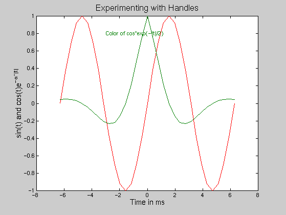
The function fplot returns the x and y coordinates used on the figure. On the other hand plot give handles to each of the curves shown on the plot. Thus we won't try to deal with handles associated with plots from fplot, but use an our example a case where we start with:
>> t=-2*pi:pi/8:2*pi;
>> hplot=plot(t,sin(t),t,cos(t).*exp(-.5*abs(t)))
hplot =
       2.0001
       5.0001
Each of the handles: hplot(1) and hplot(2) is associated with one of the curves that is shown. Note that if you have forgotten to save the handle to an object, you can find its value with the gco command. This is very handy if you have a curve (or any other object) you wish to remove from a figure, just click on it and issue the command:
>> delete(gco)
Each of the annotation commands: xlabel, ylabel, title, text, gtext and legend also returns one or more handles.
>> hxl=xlabel('time im ms')
hxl =
    6.0001
>> hyl=ylabel('sin(t) and cos(t)e^{-\alpha*|t|}')
hyl =
    7.0001
>> ht=title('Experimenting with Handles')
ht =
    8.0001
Note the very limited use of TeX characters in the label on the Y axis. This feature was used to make the Greek character for alpha and to make the exponential a superscript. It has more extensive possibilities in annotating graphs. You may also see that the exponetial part of the Y label is so small that it is unreadable in its default size and font. This is where the handles become very useful. The numeric values for the handles may be used to "fine tune" your plots. Here are a couple of examples. We may see that the font used for labeling both axes are too small. We can correct that by:
>> set(hxl,'FontSize',12)
>> set(hyl,'FontSize',12)
We can make the title even larger:
>> set(ht,'FontSize',14)
We may not like the color used to plot the first curve. To find which color was used the get command is appropriate:
>> get(hplot(1),'Color')
ans =
     0 0 1
Those three numbers give the amount of Red, Green and Blue in the color. To change to red, we will use: [1 0 0], but note that the numbers are not limited to being 0 or 1. They may also be fractions. Here is red:
>> set(hplot(1),'Color',[1 0 0])
We may even see after we use the larger font that we had a typo in the x label and need to correct it:
>> set(hxl,'String','Time in ms')
We can add text to label on of the curves in the color associated with the curve:
>> a=get(hplot(2));
>> text(-3,.8,'Color of cos*exp(-|t|/2)','Color',a.Color)
Note that a is a structure and a.color is the color associated with the second curve. Our final plot looked like:
6.4.2 Printing and Saving
Graphics Files
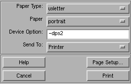
There are a variety of ways to save the graphics results that you produce in Matlab. You can of course print the window directly to a connected printer. This is easily done with the Print... Command under the File Menu at the top of the Figure Window. This File menu is shown in Figure 6.2. The selection of Print...brings up a window with lots of options.
The default settings should produce a copy of the figure on your default printer. You can chose a variety of other options such as:
You will find that after you print your figure or even if you send an image of it to a file, you will not have something that you can work with in Matlab in a different session. Matlab now allows you to recreate your figure by using the Save As... option under the File Menu. If you save your figure this way Matlab creates an m file together with a mat file. The m file can then be executed to recreate the figure. I saved Figure 6.10 calling it figure1. Here is a listing of the first part of the m file it produced:
whale% cat figure1.m
function figure1()
% This is the machine-generated representation of a MATLAB object
% and its children. Note that handle values may change when these
% objects are re-created. This may cause problems with some callbacks.
% The command syntax may be supported in the future, but is currently
% incomplete and subject to change.
% % To re-open this system, just type the name of the m-file
%   at the MATLAB prompt.
%The M-file and its associtated MAT-file must be on your path.

load figure1
a = figure('Color',[0.8 0.8 0.8], ...
'Colormap',mat0, ... 'Position',[517 351 560 420]);
b = axes('Parent',a, ...
'Box','on', ...
'CameraUpVector',[0 1 0], ...
'Color',[1 1 1], ...
...............
Looking at my home directory, I find there is a mat file produced as well as the m file.
whale% ls figure1*
figure1.m    figure1.mat
If I quit my Matlab session and come back another time, I can restore the same graph by simply typing.:
>> figure1
However, when you use the command who, you find all of the handle variables have not been reproduced. This may limit what you can do if you want to change details about the figure. If you need to make such changes, you will have to become acquainted with the commands: findobj, gca, gcf, and even more complicated set and get. I found for example that the all the handles could be determined with:
>>  Hs=findobj
Hs =
         0
    1.0000
    3.0001
    9.0001
    5.0001
    4.0001
You can see that these are not the same numeric values set when the objects were first formed.
A second topic in this section is concerned with the production of gif files for use in web pages. This section might be applied to copying a number of windows besides Matlab figures, but currently it is quite important in Matlab since there is no direct way to produce gifs or jpeg files from Figures. Here is the procedure we have used to produce most of the figures in the ceng301 and 303 web pages. If you have a whole or part of a window you want to make into a gif file, then:
Matlab can produce and manipulate two different types of figures:
graphs from programs like plot and images that might have originated
as scanned bit maps. The figure at the top of the main pages in these
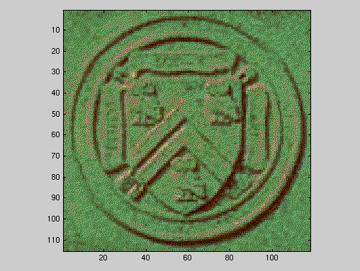
notes is an image. A copy of it is stored in
/home/ceng301/public_html/images/089-sm.jpg.
We can load that file in a Matlab session with the imread command:
>> Symb=imread('/home/ceng301/public_html/images/089-sm.jpg');
It loads as a three dimensional object with a large number of
elements.
>> size(Symb) ans = 115 118 3
If you look at a few of the elements, you see that they are
numeric:
>> Symb(1:3,1:3,1)
ans =
132 139 129
122 128 118
121 125 119
To see the images, we use:
>> image(Symb)
This produces a larger version of the figure that you have been
seeing. It looks better if it is made square:
>> axis image
You can manipulate such images in a number of ways such as by changing the colors used to map the number in the array and changing the location of the virtual light source for the image. If you produce an image that you want to save and store in a web page, you can do so with the imwrite command. It requires three arguments: the name of the image, the finame where you are going to store the data and the format you want to use. One of the allowable formats is 'jpg' (Joint Photographic Experts Group) and can be used in web pages.
Continue on to Chapter 7: More Useful MATLAB Arithmetic Functions