3.1 Discussion
3.2 Controlling Your Screen Output with disp and format
3.3 Solution of Simultaneous Equations
3.4 Data Fitting
3.5 Using Polynomials
3.6 Trial and Error Solutions
3.7 Contour Plots and a Simple Function
3.8 Easy Editing During a MATLAB Session
3.9 Communicating with Other Systems and Languages]
3.1 Discussion
The following problems illustrate many techniques helpful in solving
scientific problems. In order to make our listing of variables less
cumbersome with the disp , (for display) function, its
description here is a preliminary digression.
3.2 Controlling Your Screen Output with disp
and format
It is impossible to make the printed output from a MATLAB session
look good with just the default way of printing results. This is
particularly difficult in looking at results stored in matrices. If
you give the name of an array, you always get that name followed by
spaces and an equal sign. Even if you just give something like a
message in quotes you get ans , as the assumed name with the
spaces and equal sign. One way to avoid this is with the disp
, function. You can avoid messy extraneous printing in your error
messages with it as in the ssec2 , function. You can also
print a table of data that looks like a table as seen in the function
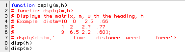
dsply.
Note that images of Matlab functions were created for these notes using a Macintosh. Color is used to designate important features of the functions and the lines are number so we can reference individual lines if needed. The colors used are:
If we follow the example to set up the values in distm: ,
>> distm=[0  0   2.3  .66

          1  2   2.7  .77

          3  6.5 2.2  .60];
we could look at it by simply:
>> distm

distm =

         0         0    2.3000    0.6600

    1.0000    2.0000    2.7000    0.7700

    3.0000    6.5000    2.2000    0.6000
but that is not very informative about its contents. The function disp , allows us to avoid repeating the name of the variable:
>> disp(distm)

         0         0    2.3000    0.6600

    1.0000    2.0000    2.7000    0.7700

    3.0000    6.5000    2.2000    0.6000
The disp , function is thus used in dsply , to allow the user to add a heading to the matrix listing:
>> dsply(distm,'      time    distance  accel     force')


      time    distance  accel     force

         0         0    2.3000    0.6600

    1.0000    2.0000    2.7000    0.7700

    3.0000    6.5000    2.2000    0.6000
We are stuck with having to adopt MATLAB's standard output format
for data, but we have made some progress. We also get an additional
blank space before the next MATLAB prompt:
'>>'. Most of these blank space
can be eliminatedby setting:
>> format compact
Then that use of the function dsply , would give:
>> dsply(distm,'      time    distance  accel     force')

      time    distance  accel     force

         0         0    2.3000    0.6600

    1.0000    2.0000    2.7000    0.7700

    3.0000    6.5000    2.2000    0.6000
We will set our environment with format compact in the rest of these notes. The format command has several uses. Here is what help shows:
>> help format

 FORMAT Set output format.

    All computations in MATLAB are done in double precision.

    FORMAT may be used to switch between different output

    display formats as follows:

      FORMAT         Default. Same as SHORT.

      FORMAT SHORT   Scaled fixed point format with 5 digits.

      FORMAT LONG    Scaled fixed point format with 15 digits.

      FORMAT SHORT E Floating point format with 5 digits.

      FORMAT LONG E  Floating point format with 15 digits.

      FORMAT SHORT G Best of fixed or floating point format with 5 digits.

      FORMAT LONG G  Best of fixed or floating point format with 15 digits.

      FORMAT HEX     Hexadecimal format.

      FORMAT +       The symbols +, - and blank are printed

                     for positive, negative and zero elements.

                     Imaginary parts are ignored.

      FORMAT BANK    Fixed format for dollars and cents.

      FORMAT RAT     Approximation by ratio of small integers.


    Spacing:

      FORMAT COMPACT Suppress extra line-feeds.

      FORMAT LOOSE   Puts the extra line-feeds back in.
Suppose you want to see the elements in the vector formed by:
>> v=exp(-10*(1:5))

v =

   1.0e-04 *

    0.4540    0.0000    0.0000    0.0000    0.0000
Obviously, that does not give very much information in the default SHORT format mode. Now let's try two other options:
>> format long

>> disp(v)


   1.0e-04 *

  Columns 1 through 3

   0.45399929762485   0.00002061153622   0.00000000093576

  Columns 4 through 5

   0.00000000000004   0.00000000000000


>> format short e

>> disp(v)

   4.5400e-05   2.0612e-09   9.3576e-14   4.2484e-18   1.9287e-22
The LONG mode gives more decimal places but again does not cover
the entire range in our vector. The SHORT E , or LONG E , option is
required to see what has really been stored in v.
We will impose format compact in the rest of the notes and
occasionally use other formats to show what has been produced.
3.3 Solution of Simultaneous Equations
Scientific problems always seem to involve the solution of
simultaneous linear equations. For a few equations (two or three at
most) this may be done by hand. For more than three equations it is
advisable to use a computer. We will look at the MATLAB solution of
such equations by way of the example: Solve for x1, x2, and x3
satisfying:
   3.5x1  +   2x2            =  5

  -1.5x1  + 2.8x2 + 1.9x3    = -1

          - 2.5x2   , 3x3    =  2
We have already seen how to do this, but it is worthwhile repeating to make sure we have not forgotten the details. In MATLAB the solution would be found as seen next:
>> a=[3.5  2   0

     -1.5  2.8 1.9

      0   -2.5 3];

>> b=[5 -1 2];

>> a\b'

ans =

    1.4421

   -0.0236

    0.6470
The answer may be interpreted as: x1 = 1.4421 , x2 =-0.0236 , x3 = 0.6470 . Now see that this looks even better with disp:
>> disp(a\b')

    1.4421

   -0.0236

    0.6470
3.4 Data Fitting
A second common operation in scientific work is the fitting of
experimental data by means of an approximating polynomial. The
following set of data gives the values for yi measured at values of
xi.
	i	xi	yi

	1	0	1.9

	2	2	2.9

	3	4	4.7

	4	5	5.1

	5	9	8.0
We wish to find various polynomials that might be used for smoothing this data or interpolating between points in the table. First we will try a linear approximation. This means we want to find c0 and c1 such that
y ~= c0 + c1x
at each of the data points. Since there are five points and only two unknowns this is very unlikely. MATLAB has a function called polyfit , that finds the coefficients that ``best" fit the data with a polynomial in the least squares sense. The function requires three arguments: x, y and n : x and y are vectors of data and n is the order of the polynomial. We see it used in the session:
>> x=[0 2 4 5 9];

>> y=[1.1 2.9 4.7 5.1 8];

>> cl=polyfit(x,y,1);

>> disp(cl)

    0.7587    1.3252
Coefficients returned by the function are always listed in the order of decreasing powers of x . Thus the ``best" linear approximation is:
y ~= 0.7587x + 1.3252
The procedure for finding the ``best" quadratic fit is shown next:
>> cq=polyfit(x,y,2);

>> disp(cq)

   -0.0176    0.9199    1.1232
The best quadratic fit was thus found to be:
y ~= - 0.0176x2 + 0.9199x + 1.1232
3.5 Using Polynomials
We will now look at methods that allow polynomial coefficients like
cl and cq to be used in MATLAB for interpolation, smoothing and
comparison with experimental data.
The function polyval , is the main tool for finding the value
of:
for either a single value of x or at each x in a vector or matrix. If
we continue the session from Example 2, we see that the linear
approximation can be compared to the original data by:
>> yla=polyval(cl,x);

>> disp(yla)

    1.3252    2.8426    4.3600    5.1187    8.1535
and the quadratic approximation by:
>> yqa=polyval(cq,x);

>> disp(yqa)

    1.1232    2.8927    4.5217    5.2834    7.9790
A table to compare the linear approximation is found by:
>> ela=y-yla;

>> mla=[x;y;yla;ela]';

>> dsply(mla,'       x         y        yla       ela')

       x         y        yla       ela

         0    1.1000    1.3252   -0.2252

    2.0000    2.9000    2.8426    0.0574

    4.0000    4.7000    4.3600    0.3400

    5.0000    5.1000    5.1187   -0.0187

    9.0000    8.0000    8.1535   -0.1535
Similarly the quadratic approximation looks like:
>> eqa=y-yqa;

>> mqa=[x;y;yqa;eqa]';

>> dsply(mqa,'       x         y        yqa       eqa')

       x         y        yqa       eqa

         0    1.1000    1.1232   -0.0232

    2.0000    2.9000    2.8927    0.0073

    4.0000    4.7000    4.5217    0.1783

    5.0000    5.1000    5.2834   -0.1834

    9.0000    8.0000    7.9790    0.0210
The average absolute error in the linear fit may be found by:
>> disp(sum(abs(ela))/5)

    0.1590
This may be compared to the quadratic fit by:
>> disp(sum(abs(eqa))/5)

    0.0827
There is also a MATLAB function called polyder , that allows the derivative of a polynomial to be found. Here is what it gives when we apply it to the two sets of polynomial coefficients we found:
>> polyder(cl)

ans =

    0.7587

>> polyder(cq)

ans =

   -0.0351    0.9199
These show that the derivative of 0.7587x + 1.3252 is 0.7587 and the derivative of:
- 0.0176x^2 + 0.9199x + 1.1232 .
is -0.0351x + .9199 . In these cases we could see by inspection
what the derivatives of our polynomials should be, but for more
complicated cases, this function can be very useful.
MATLAB's graphics allow us to see a
comparison of the polynomial approximations with the original data in
our example:
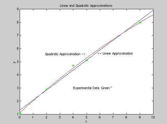
>> xs=0:.1:10;

>> yl=polyval(cl,xs);

>> yq=polyval(cq,xs);

>> plot(xs,yl,xs,yq,'r')

>> hold
Current plot held
>> plot(x,y,'g*')

>> title('Linear and Quadratic Approximations')

>> xlabel('x')

>> ylabel('y')

>> text(4,3,'Experimental Data Green *')

>> gtext('<- Linear Approximation')

>> gtext('Quadratic Approximation ->')

>> print
Here is the plot:
Figure 3.1 Approximations to Experimental Data
|
|
3.6 Trial and Error
Solutions
The solution of nonlinear problems nearly always requires the use of
a trial and error procedure to find a close approximation to a root
of an equation. Roots of polynomials may be found with the MATLAB
function roots , demonstrated in the chapter on programs.
Other functions could be approximated by polynomials and then roots
found as shown in that same chapter.
A general purpose program that will find a root of a single equation
by one version of the secant method is called ssec2. We will
demonstrate it by finding the roots of the
cubic equation:
x3 - 2x2 - 4.25x + 7.5 = p(x) = 0
Two functions are actually used: ssec1 , and ssec2.
, These functions are described more fully in the chapter on MATLAB
functions. The second of these programs uses the first one. The
ssec1 , program takes two ``guessed" values for x and finds
the value of f(x) at each. Then it predicts a new value that would
give 0 for a result if the function were linear. The ssec2 ,
program starts with two values for x and uses ssec1 , up to
nmax , times to try to make the difference between two successive
guesses less in magnitude than erc. Each time after ssec1 , is
used, the value it predicts is used to replace the ``oldest"
guess.
We will concentrate here on the use of ssec2, , since that is
the one that will actually find a root of an equation. The comments
in the function may be seen by:
>> help ssec2


  function x=ssec2(xs,fx,c,erc,nmax)

  xs gives an interval to seek a solution to f(x) = 0 in.

  fx is a character vector that tells how to find f(x).

  c is a vector of parameters in f(x)

  erc gives the difference between successive values of x

  allowed when convergence is deemed to be achieved.

  nmax is the maximum number of trials, before quitting.

  If erc and nmax are not given, then the program uses:

     erc=.0001 and nmax=10

  If only two arguments are given, c is set to null.

  The program uses the function ssec1 for each iteration.

  Example 1:>> cs=[1 -2 -4.25 7.5];

            >> disp(ssec2([2 3],'polyval(c,x)',cs,.0001,10))

  Example 2:>> ssec2([3 4],'sin(x)')
The first example shown in the comments for the function finds one root of the cubic in this discussion. We can see that it finds the root at x = 2.5 by trying it:
>> cs=[1 -2 -4.25 7.5];

>> disp(ssec2([2 3],'polyval(c,x)',cs))

    2.5000
Other roots may be found as seen next:
>> disp(ssec2([0 2],'polyval(c,x)',cs))

    1.5000


>> disp(ssec2([-3 -1],'polyval(c,x)',cs))

   -2.0000
Of course all these could also have been found with roots, by simply:
>> disp(roots(cs))

    2.5000

    1.5000

   -2.0000
The program ssec2 , does not always give a root in the specified interval and sometimes fails to converge if the initial interval is too large as shown in the next session.
>> disp(ssec2([-5 0],'polyval(c,x)',cs))

    1.5000


>> disp(ssec2([2 5],'polyval(c,x)',cs))


*******************************************************

* ssec2 did not converge, xl:    2.5155 xr:    2.4987 *

*******************************************************

    2.4987
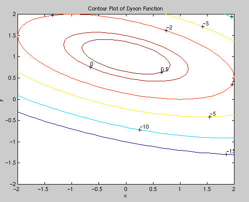
3.7 Contour Plots and a Simple Function
Contour plots frequently give the user a picture of a function's
behavior particularly in the vicinity of stationary points. The
function:
f(x,y) = 2 - [(x-1)2 + 4(y-1)2 + 2xy]
has a stationary maximum near (0,1). Here is a MATLAB function that will give a matrix of values of the function for vector of x and y :
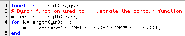
Note particularly that as vectors are added to the matrix, the
last value of y is used first and then we work toward the first value
of y .
The following session gave a contour plot of this function for both x
and y in the interval (-2,2):
>> xs=-2:.1:2;

>> ys=xs;

>> m=prof(xs,ys);

>> cs=contour(xs,ys,flipud(m),[-15 -10 -5 -2 0 .5]);

>> clabel(cs)

>> xlabel('x')

>> ylabel('y')

>> title('Contour Plot of Dyson Function')
The function flipud, which flips a matrix upside down, is
used with the contour command in order to make the graph
appear right-side-up. (This is because in MATLAB 4, the appearance of
the graph has been flipped in the up/down direction.)
Figure 3.2 A Contour Plot
|
|
3.8 Easy Editing During a MATLAB Session
If you have been trying some of the example problems in these notes,
you have probably discovered that it is difficult to type an entire
line without error. When you start generating your own commands you
will find it even more difficult to type in exactly what you want the
first time you try something.Fortunately, MATLAB provides a means for
trying out corrections on a line-by-line basis. On the right side of
the SUN keyboard, in the lower part of the R-functions key pad, there
are four keys with black arrows --- called cursor keys. The
up-pointing arrow moves the `line to be selected' upward toward
earlier commands in the MATLAB session; the down arrow moves it
downward. Each time you press either of these arrows, a new line
appears at the bottom of your session ready to be executed with a
RETURN . To edit this line, press the left arrow to move the cursor
letter-by-letter toward the start of the line until the point is
reached where you want to erase, change or insert one or more
characters. Alternating left and right arrows allows you to edit any
part of the line. When you are done press RETURN.
3.9 Communicating with Other Systems and Languages
In this section we will examine ways to use MATLAB with other
languages such as FORTRAN and C. MATLAB has several shortcomings such
as:
a) its lack of speed in looping operations,
b) its limited character handling ability,
c) its limited ability to read data from files,
d) its lack of multidimensional arrays beyond matrices,
e) its limited control over windows and menus.
Both FORTRAN and C can now be used to create functions to be
called in MATLAB that can give tremendous improvements in speed as
well as the other limitations listed. Section I.7.4 in the MATLAB
User's Guide shows how one can develop a FORTRAN version of a
function called yprime that can speed up the solution of a
model of an orbiting object.
An easier way to use FORTRAN programs in MATLAB is by simply using a
FORTRAN program to create a data file that can be read into MATLAB.
The program tprop2 is stored in ~ceng301/prog4, so
chemical engineering students can execute it by simply typing its
name. It can be used to created a file of thermodynamic data that can
then be loaded into a MATLAB session and plotted. For an illustration
of its use, see the
Ceng 301 Notes:
Data stored in the file created with tprop2 may be displayed in MATLAB with the program tplot1:
>> load water.dat

>> help tplot1

  function tplot1(m,com,n0,n1,n2,fx,fy)

  Turns the plot hold OFF.

  Plots column n2 vs column n1 in m with lines of constant

     column n0 connected by solid lines and marked with

     different symbols.

  Adds title and axis labels.

       Argument List

  Arg   Specifies

   m   matrix of data from thermo properties FORTRAN program.

  com  name of the compound in single quotes.

   n0  column with data to sort on: 1 is p, 2 is t

   n1  column of data for x axis

   n2  column of data for y axis

   fx  fraction to shift text in x direction.

   fy  fraction to shift text in y direction.

       If these are not given, 0.1 is used for each.

        Values of nk

   k    Specifies

   1   Pressure kPa

   11  log(Pressure)

   2   Temperature C

   3   Volume m3/kg

   4   Entropy kJ/kg-K

   5   Enthalpy kJ/kg

   6   Int. Eng. kJ/kg

   7   Gibbs Eng. kJ/kg
We can plot and then print the data by:
>> tplot1(water,'Water',1,2,5, 0.3, .07)

>> print
Here is what we get:
Figure 3.3 Steam Enthalpy Plot
|
|
It can be seen from this figure that water boils at about
99°C at a pressure of 100 kPa and at about 212°C when the
pressure is 2000kPa. These values agree with those in steam
tables.