
<! Page Header >
<! Main Body > The following topics will be discussed:
5.1 The mods2.m File
5.2 The start301c Module
5.3 The mix Module
5.4 The split Module
5.5 The sep Module
5.6 The react Module
5.7 The Displays Modules : show1,show2
The Matlab Mass Balance Modules simplify calculations involved in simulating the behavior of steady state chemical systems. They require that the parameters that specify all units be given in a very simple form. In particular the flow of all streams into each unit must be known. If we do not know the flow rates of all compounds into each unit, we are forced to use some trial and error procedure to complete our simulation. Even simple processes that are part of a system that includes recycle demand that we use trial and error processes to solve them with the Matlab modules. This in not too bad as long as we need to solve for a single unknown by trial and error. It can lead to very difficult procedures if we need to solve for many unknowns such as the flows of all compounds in a recycle stream.
This chapter will show how Mass Balance Modules can be written in Maple. Maple has the definite edge over Matlab when it comes to handling this problem in a program. In our Matlab modules, missing data was handled by inserting NaNs. At least that gave a warning if you tried to calculate something that needed the data. It would simply come out as NaN and you would know to go search for the missing data. In Maple we will insert names for missing data and should be able to see what caused anything to be given as a symbolic rather than a numeric result. When we complete our description of the complete process, we can then set up equations that we need to solve in order to complete our simulation. We will find that for certain problems this can greatly improve our chances of finding an analytical soultion to our mass balance problems.
The Maple Modules will require the use of linear algebra so the linear algebra package will always be invoked at the beginning of a simulation. If you have questions about this package, review chapter 3 or use the help command to find out more about it and the commands that are useful in manipulating arrays. All the mass balance modules found in Matlab have been converted into Maple modules as well :
The file /home/ceng301/maple/mods2.m executes the necessary commands to load the linear algebra package and read all the mass balance modules (these will be discussed in later sections in this chapter). Therefore, with one command, all the modules are available for usage and users can quickly start up sessions in Maple. In order to set up a Maple work session for use with the mass balance modules, the following command needs to be issued:

The start301c module is the Maple variant to start301a. A FORTRAN program, start301c generates a Maple V program that can be executed in order to set up all the data required for the mass balance modules. start301c needs to be run at a UNIX prompt (NOT at the Maple prompt). The file that is generated by start301c can then be used in Maple.
The following examples illustrate the usage of start301c:
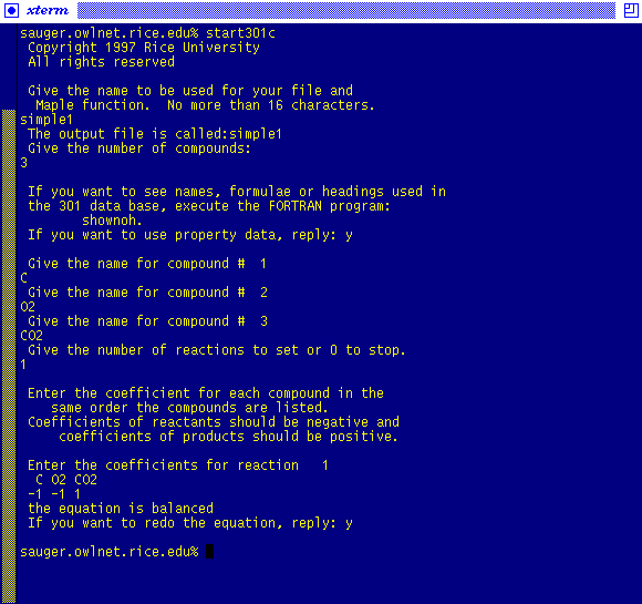
Therefore, start301c has created the Maple program:
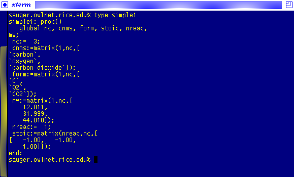
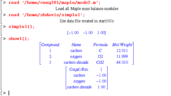
With the simple1 file created, the program can be run in a Maple Vr4 session:
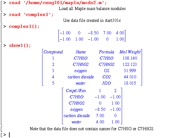
Reacting cresol (C7H8O) with oxygen to form benzoic acid with a side reaction to complete combustion. The data program complex1 was created by start301c as described above. However, C7H8O nor the reaction product C7H6O2 is in the data bank. Therefore the data file will yield the following result:
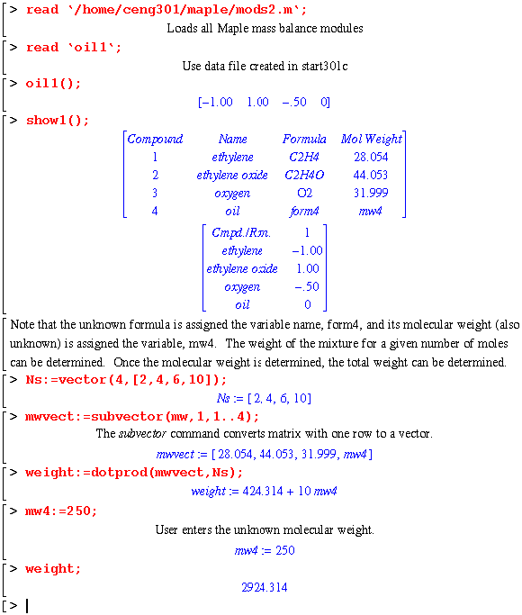
An oil of unknown composition is used in cooling the partial oxidation of ethylene to ethylene oxide. Once again, start301c was used to set up the data file, oil1:
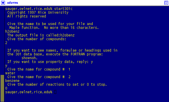
Using start301c, a water and benzene system is set up. Maple will be used to determine the vapor pressure. In addition, the heat capacity data will be converted into polynomials to determine the enthalpy difference. The property data in the sdata file in the ceng301 directory will be used.
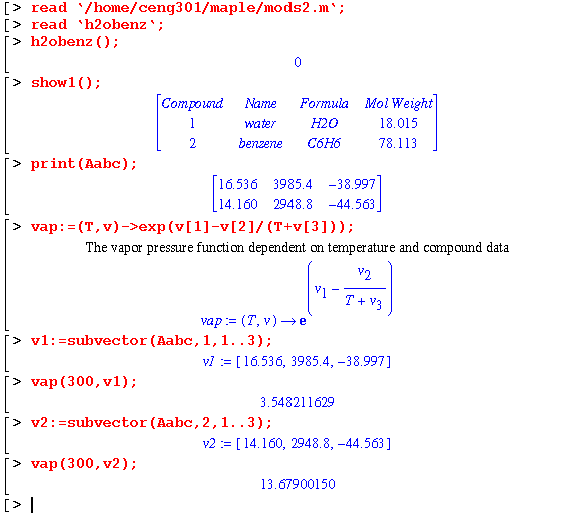
The vapor pressure of each compound can be determined by creating a function as illustrated:
In order to determine the enthalpy difference, the heat capacity data needs to be converted into polynomials. The matrix containing heat capacity data is separated into vectors prior to polynomial conversion and integration.
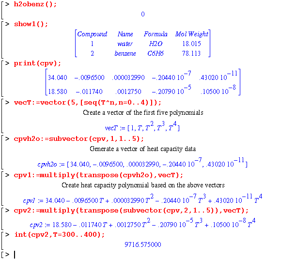
Maple can generate the heat capacity polynomials simultaneously for both compounds. In addition, if the property data is missing, Maple just substitutes a variable name until the data is defined:
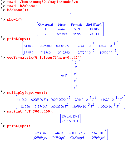
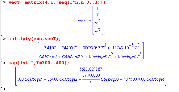
The start301c module is vital to the usage of the mass balance modules since it sets up all the variables. In addition, with the nice feature of Maple to assign variable names for unknown data, the system can still be analyzed.
Before any of the modules can be executed, two things are required : (1) an array called Ns must be set up to hold the flows for each stream and (2) the mods2.m file must be loaded to set up all the modules. The mix module mixes streams in the in1 array to form the outlet stream, out:
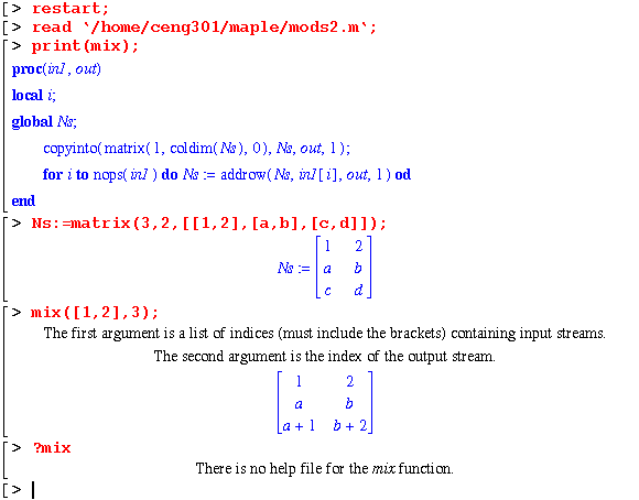
Note that the mix module does the same thing in Maple as in Matlab; but it also does more. The flow of each compound in stream 2 can be given as symbols. The flow in stream 3 carries these symbols along.
The split module splits the input stream, in1, into the out stream array given outlet stream fraction, t.
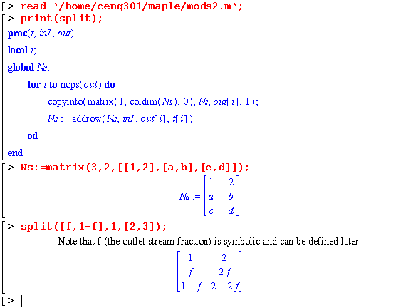
As you can see in the example the fraction of stream 1 that is sent to stream 2 can be given a symbolic value. This is exactly what you want in many simulations. Note that the first and last arguments to split must be lists. They must also have the same number of elements.
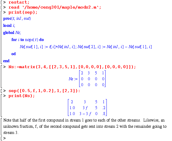
The sep module models a separator by separting the in1 stream into outlet streams, out, with the fraction, t, of each compound going to the outlet streams:
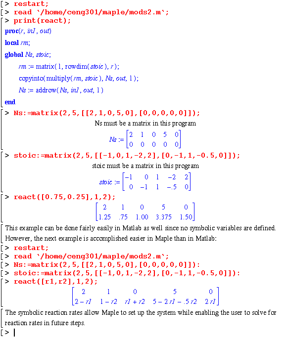
The react module simulates a reactor using stoichiometric coefficients stored in the variable, stoic, and reaction rates, r:
5.7 The Display Modules : show1,show2
The display modules show1 and show2 are used frequently to display the information contained in all the arrays. The show1 lists the compounds names, formulas, molecular weights, and all reaction stoichiometry defined by start301c. The show2 function was designed by Matt Hayenga to make use of the data created with start301c by listing:
<! Manual Options >